ASSEMBLY LAYERS
Overview
Assembly layers contain block representations of the components on the board, along with their reference idents in the middle. They are often used for population of the PCB, particularly when the silkscreen references have been selectively removed due to space constraints.
The Assembly Data
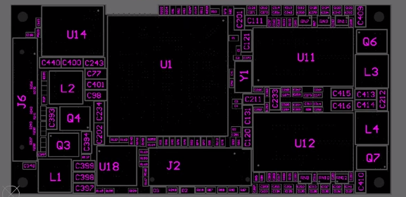
Example of Assembly Drawing.
Assembly data is auto-generated by the Proteus software. The required information is simply:
- Component Part References.
- Component Occupancy Definitions.
- Pin 1 Indicators.
Component Occupancy Definition
The occupancy definition for the part is generated based on the following, in order of decreasing priority:
- Contents of the relevant Assembly Layer in the footprint if present.
- Contents of the courtyard if present (occupancy layer).
- Simple geometric bounding box for the component.
Pin 1 Indicators are applied automatically in cases 2 and 3 above. Where Assembly Layer content is explicitly present it is deemed to be complete and correct and no additions (such as pin 1 indicators) are made by the software.
The occupancy definition is used as the courtyard for the part on the assembly drawing and the component part reference is then centred and oriented inside it.
It doesn't matter if you choose to hide the component part reference on the silkscreen layer.
Pin 1 Indicators
If the component has assembly graphics then no pin 1 indicator is drawn because it is assumed that it exists on the assembly graphic (often pin 1 indication is a chamfer or diagonal drawn on a box corner).
If the component has no assembly graphics then an indicator is placed automatically as a small dot. Proteus chooses the pin to mark as follows:
- The pin numbered 1, wherever the package has one.
- The pin numbered A1, to cater for the grid based numbering used by BGA packages. This is only accepted on packages of more than two pins, so that a two-pin part with an A1 pin is not mistaken for a BGA.
- On a two-pin package, the pin named C, K or -. This marks the cathode of a diode or the negative terminal of a polarised capacitor, which is the terminal an assembler needs to identify.
Single-pin packages such as mounting holes and fiducials are never marked.
Working with the Assembly Plot
There are two ways to manage and work with Assembly Plots.
- Automatic. Do not include assembly layer data in packages but do include an occupancy graphic. This is what happens by default with all imported parts.
- Manual. Draw assembly layer data and pin 1 indicator on a decomposed package and then re-make the package into your libraries.
If you draw assembly layer data, make sure to draw everything you want including the pin 1 indicator. If any assembly data exists for a component then Proteus assumes it is all present and correct.
In practice, it is far more likely that the automatic mode is fastest and easiest to work with. Note that pin 1 indicators can be removed en-masse (for example, for non-polarised passives) by adding the ASSEM_NO_MARK property in Design Explorer. This is discussed in more detail below.
However being able to draw custom assembly graphics gives you total control of size and style. You may choose to use this option for the odd part where a simple occupancy graphic is less suitable.
See Also:
Drawing Assembly Graphics for a Package
Let us take an example. We have an electrolytic capacitor package for which there is no occupancy layer definition and no assembly layer content. The result is that a simple bounding rectangle is used for the assembly plot which is not ideal.
To override this behaviour we need to add content to the package.
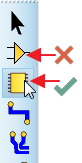
It's a very common mistake to try and edit the component. Must be the package.
So, we switch to package mode as in the picture above, find the part we want and place one where there is space. Then:
- Right click on the package and select decompose from the context menu.
- Place the appropriate 2D graphic object (for example a circle) on the assembly layer around the part.
- Add a pin 1 indicator if desired.
- Drag a selection box around everything, right click and select Make package.
- Choose to update all instances on the layout when prompted to reflect your change.
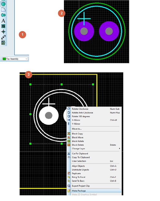
Adding Assembly Information to a part.
It is worth noting that it is extremely unlikely that you will have to do this. As far as we can tell almost all imported parts from our partners include occupancy layer definitions (courtyard) which will be used if no Assembly layer data is present.
While assembly data is included in the data set for most imported parts we have chosen to strip it from the parts in Proteus because it is inconsistent, very often incomplete and sometimes completely wrong.
Viewing the Assembly Plot in the Editor
The Assembly plot can be viewed by setting up a colour set in the view layer dialogue.
Open the View Layers dialogue either from the View Menu command or, more easily, by clicking on the main status bar.
Press the New button beside the Colour Sets and give a sensible name (for example, Top Assembly).
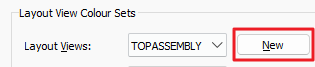
Creating a new layout view colour set named TOPASSEMBLY.
Select None to clear all the layers and then tick the Draw Component Assembly checkbox, turn on Edge Layer (under the Physical Layers tab) and lastly Top Assembly Layer (under the Data Layers tab). Assign a keyboard shortcut (number 4 in our example).
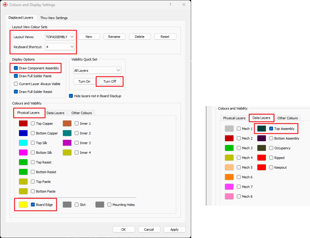
Selecting Draw Component Assembly, the Edge layer and the Top Assembly layer for the new colour set.
Hit OK to exit the dialogue form and store your settings. The editing window should now show your Assembly plot.
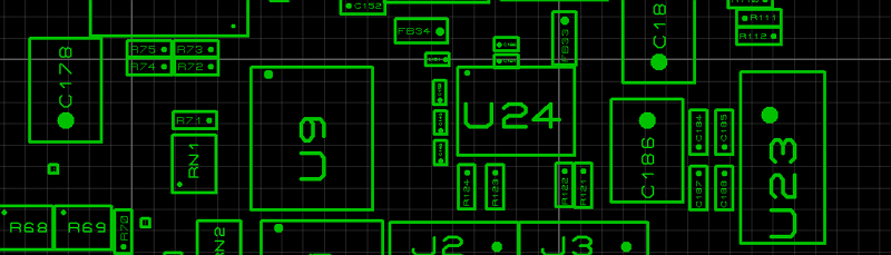
The editing window showing the top assembly plot.
You will almost certainly want to open up the View Layers dialogue again and assign your main view (for example, BLACK PAPER) to number 1 if you have not already done so. Hit OK to exit the dialogue form again.
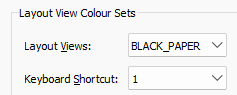
Assigning the main board view to keyboard number 1.
You should now be able to switch between views with a keypress. Note that this scheme is highly extendable and extremely useful generally. The reason for assigning number 4 to top assembly view is mostly that number 1 is the full board view, number 2 is assigned to TOP VIEW and number 3 to BOT VIEW, where one side of the board is turned off.
Switching back to Assembly view note that:
- You can add graphics such as dimensions or text directly to the assembly layer.
- You can add dimensions, text, legends and so on to one or more mechanical layers and then include them in your Assembly view by checking the appropriate visibility checkbox.
Output of Assembly Layers
A component that is not fitted in the currently selected Assembly variant still appears on the Assembly Drawing, but it is drawn with a diagonal cross through its box so that the assembler can see at a glance that the position is to be left empty.
Manufacturing Output
Assembly layers can be included as standard with both the Gerber X2 and the ODB++ Export formats. When using the Gerber X2 format, they import into the Gerber Viewer as Top Assembly and Bottom Assembly layers under their own names, as shown below.
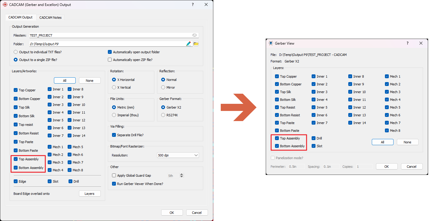
Top Assembly and Bottom Assembly selected for CADCAM output, then listed under their own names when the fileset is loaded into the Gerber Viewer.
It follows that you can then either view only the required assembly layer by turning off all the other layers in the Gerber viewer, or you can disable the Assembly layers while viewing other board data. Layer visibility in the Gerber viewer is controlled either by clicking on the main status bar or from the View menu.
It can be useful to first generate the Gerber X2 fileset and then, if required, output the print or PDF from the resulting Gerber view where you can visualise the output.
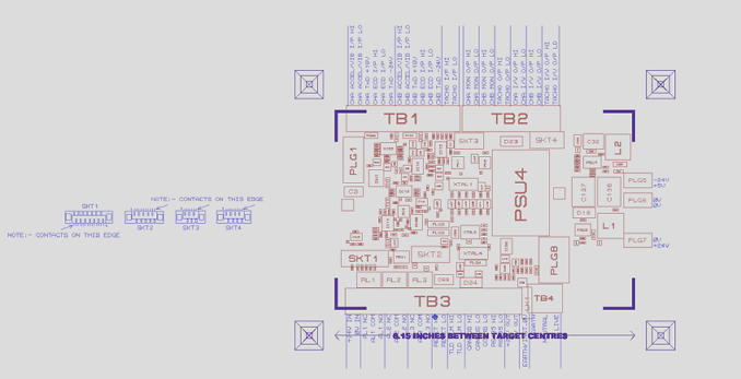
Example View of Top Assembly with Mech info in the Gerber Viewer.
Printed/Documentation Output
Assembly plot is one of the modes offered in the output dialogue forms. You can therefore opt to include more data, such as board dimensions on a mechanical layer as well as additional copper features should you need to.
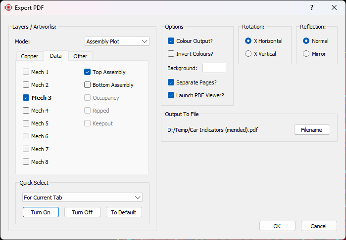
Generating a PDF for top assembly and mech data.
You can also export assembly drawings in the PCB manufacturing report in the Project Notes module.
A small pin 1 indicator is output with the assembly plot but will not be visible if the pads are included in the output because it is often situated under a pad. If you need to see pin 1 indicators you should turn off the relevant copper layer so that the pads do not obscure the indicators. Pin 1 indicators may still be difficult to spot on very small ICs and would be better viewed in a PDF where you can zoom in.
Pin 1 Indicators
First, a recap of how the assembly plot is constructed:
- If a component package has any data on the assembly layer then that data is used. The software does not attempt to add to it or take away from it.
- If a component package has no data on the assembly layer but has an occupancy definition on the Occupancy layer then that is used as the component courtyard boundary. Proteus will place a pin 1 indicator.
- If there is neither assembly data nor occupancy definition then a simple bounding box is used for the component boundary. Proteus will place a pin 1 indicator.
In summary, if you add assembly layer data to packages make sure you add the pin 1 indicator as well, because Proteus will not.
Removing Pin 1 Indicators
In the default situation a pin 1 indicator (or BGA ball A1 indicator) is provided for all components. In the case of non-polarised passives you may want to remove this for clarity. You do this by adding the following property to every relevant component:
ASSEM_NO_MARK=TRUE
The value matters. Proteus reads the property and suppresses the marker only when the value is TRUE, T, 1 or ON. Setting the property to FALSE, or removing it altogether, restores the marker.
Let us look at an example of how you might do it on a design. Start by opening Design Explorer, choosing the search tab and selecting resistors.
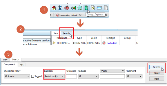
Generate a listing of all Resistors in Design Explorer.
This should give you a listing of all the resistors on the design in a grid. Next, view the property columns via the command on the View Menu in Design Explorer. Delete the text in the box and type in the property we want before hitting ENTER to add it.

Adding the property here makes it a column in the grid and therefore allows us to set its value.
You will notice that an extra column appears in the grid with this property as the column title. All we need to do now is apply the property value. Type TRUE in the first box and then hold the left mouse button down inside the typed cell and drag it down the rest of the cells to copy the value.
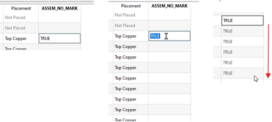
Either type, copy and paste or just drag the mouse down to copy the cell results into other grid cells.
That is it. Rinse and repeat as needed. You can also add the property manually on the schematic by copying it into the Edit Component text field:
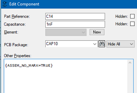
Adding the ASSEM_NO_MARK property in the Edit Component dialogue.
When entering properties manually (that is, not through Design Explorer) curly braces around the property hide the text on the schematic.
Finally, if this is something that you will always want to happen it is worth setting up once in your libraries rather than applying to every design. To do this, open Library Manager, select the library you want and then click on the Edit Library button.
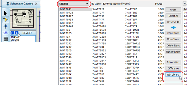
Edit the Library directly in Library Manager.
Now the procedure is very similar to Design Explorer. Create the property and select it for viewing, which will add a column to the grid listing of components.
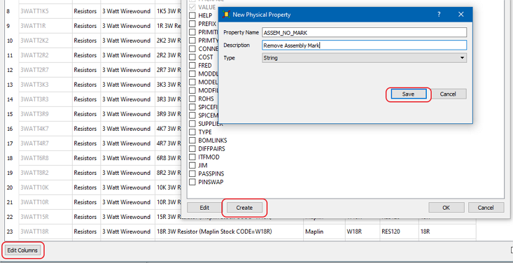
Adding the property as a column in the Library Manager grid.
Then, set one cell value to be TRUE and click drag the mouse down to set the rest of the column values.
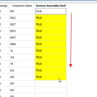
Setting the property value for every part in the library.